Basic Fitting Mode

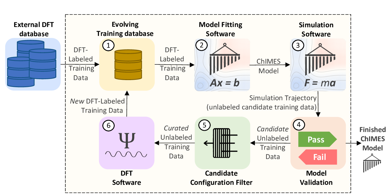
Fig. 1: The ChIMES Active Learning Driver Workflow.

The “active learning” portion of the ALD largely entails intelligent strategies for selecting candidate unlabeled training data (step 5 in the schematic above). However, the ALD can also be run in a simpler iterative refinement scheme, which is quite efficient for low complexity non-reactive problems. In this page, a single-state-point fit is demonstrated using VASP, and all additional options for fitting in this model are overviewed.

---

Example Fit: Molten Carbon

Note

Files for this example are located in ./<al_driver base folder>/examples/simple_iter_single_statepoint

In this section, an example 3-iteration fit for molten carbon at 6000 K and 2.0 g/cc is overviewed. The model will include up-to-three body interactions with the following hyperparameters. For more information on ChIMES hyperparameters and selection strategies, see:

• The ChIMES LSQ code manual (link)

• R.K. Lindsey, L.E. Fried, N. Goldman, JCTC, 13, 6222 (2017) (link)

• R.K. Lindsey, L.E. Fried, N. Goldman, JCTC 15 436 (2019) (link)

Hyperparameter	Value
2-body order	12
2-body outer cutoff	3.15
3-body order	4
3-body outer cutoff	3.15
inner cutoff	0.98
Morse lambda	1.25
Tersoff parameter	0.75

Input Files

The neccesary input files and directory tree structure are provided in the example folder, i.e.:

$: tree
.
├── ALL_BASE_FILES
│   ├── ALC-0_BASEFILES
│   │   ├── fm_setup.in
│   │   ├── liquid_6000K_2.0gcc.xyzf
│   │   └── traj_list.dat
│   ├── CHIMESMD_BASEFILES
│   │   ├── bonds.dat
│   │   ├── case-0.indep-0.input.xyz
│   │   ├── case-0.indep-0.run_md.in
│   │   └── run_molanal.sh
│   └── QM_BASEFILES
│       ├── 6000.INCAR
│       ├── C.POTCAR
│       └── KPOINTS
└── config.py

Briefly:

• ALL_BASE_FILES/ALC-0_BASEFILES contains files specifying how step 2 of figure 1 should be run, i.e., model hyperparameters (fm_setup.in), a list of training configuration files (traj_list.dat), and in this case, a single initial training configuration file (liquid_6000K_2.0gcc.xyzf).

• The ALL_BASE_FILES/CHIMESMD_BASEFILES directory contains files specifying how step 3 of figure 1 should be run, i.e., simulation parameters (case-0.indep-0.run_md.in), initial system configurations for simulation (case-0.indep-0.input.xyz), and hyperparameters for simulation output post-processing (bonds.dat VERIFY RUN MOLANAL IS NEEDED … CAN MOVE IT INTO AL DRIVER FILES).

• The ALL_BASE_FILES/QM_BASEFILES directory contains files specifying how step 6 of figure 1 should be run, i.e., quantum calculation instructions (6000.INCAR), psuedopotential files (C.POTCAR), and a K-point file (KPOINTS).

• the config.py provides high-level instructions on how all steps in figure 1 should be run.

A detailed description of the files in ALL_BASE_FILES/ALC-0_BASEFILES and ALL_BASE_FILES/CHIMESMD_BASEFILES can be found in the ChIMES LSQ manual.

Tip

In fm_setup.in, 3-and-greater polnomial orders are given as n+1. In the following example, a 3-body order of 4 is desired, hence a value of n+1 = 5 is given in the example fm_setup.in.

Contents of the config.py file must be modified to reflect your absolute paths prior to running this example, i.e. on the lines highlighed below:

# Configured for seamless run on LLNL-LC (Quartz)

################################
##### General options
################################

ATOM_TYPES     = ["C"]
NO_CASES       = 1

DRIVER_DIR     = "/usr/WS2/rlindsey/test_cp2k/al_driver/"
WORKING_DIR    = "/usr/WS2/rlindsey/test_cp2k/al_driver/examples/simple_iter_single_statepoint/"
CHIMES_SRCDIR  = "/usr/WS2/rlindsey/test_cp2k/chimes_lsq/src/"

# Job submitting settings (avoid defaults because they will lead to long queue times)

CHIMES_BUILD_NODES = 2
CHIMES_BUILD_QUEUE = "pdebug"
CHIMES_BUILD_TIME  = "01:00:00"

CHIMES_SOLVE_NODES = 2
CHIMES_SOLVE_QUEUE = "pdebug"
CHIMES_SOLVE_TIME  = "01:00:00"

################################
##### Single-Point QM
################################

VASP_EXE = "/usr/gapps/emc-vasp/vasp.5.4.4/build/gam/vasp"
VASP_QUEUE  = "pdebug"
VASP_TIME    = "01:00:00"
VASP_NODES   = 2
VASP_PPN     = 36
VASP_MODULES = "mkl intel/18.0.1 impi/2018.0"

Running

Depending on standard queuing times for your system, the ALD could take quite some time (e.g., hours) finish. For this reason it is generally, it is recommended to run the ALD from within a screen session on your HPC system. To do so, log into your HPC system and execute the following commands:

$: cd /path/to/my/example/files
$: screen
$: unbuffer python3 /path/to/your/ald/installation/main.py 0 1 2 3 | tee driver-0.log

If unbuffer is not implemented on your HPC system, use python3 -u instead. Note that in the final line above, the sequence of numbers indicates 3 active learning cycles will be run (i.e., the 0 is ignored but required when simple iterative refinement mode is selected), and | tee driver.log sends all output to both the screen and a file named driver.log.

Tip

To detach from the screen session, execute ctrl a followed by ctrl d. You can now log out of the HPC system without dirupting the ALD. Be sure to take note of which node you were logged into. You can reattach to the session later by logging into the same node and executing screen -r

Inspecting the output

Warning

When running the Active Learning Driver, ALWAYS read through the resulting log file carefully. If driver sets a large number of default parameters if the user does not specify them manually, which may or many not be conducive to the user’s end goal. The top portion of the log file tells the user every default that it sets.

Once the ALD has finished running, execute the following commands:

$: cd /path/to/examples/simple_iter_single_statepoint/
$: for i in {1..3}; do cd ALC-${i}/GEN_FF; paste b_comb.txt force.txt > compare.txt; cd -; done

Then, plot ALC-{3,2,1}/GEN_FF/compare.txt with your favorite plotting software. This file may contain force, energy, and stress values. For a force-only fit, the resulting figure should look like the following:

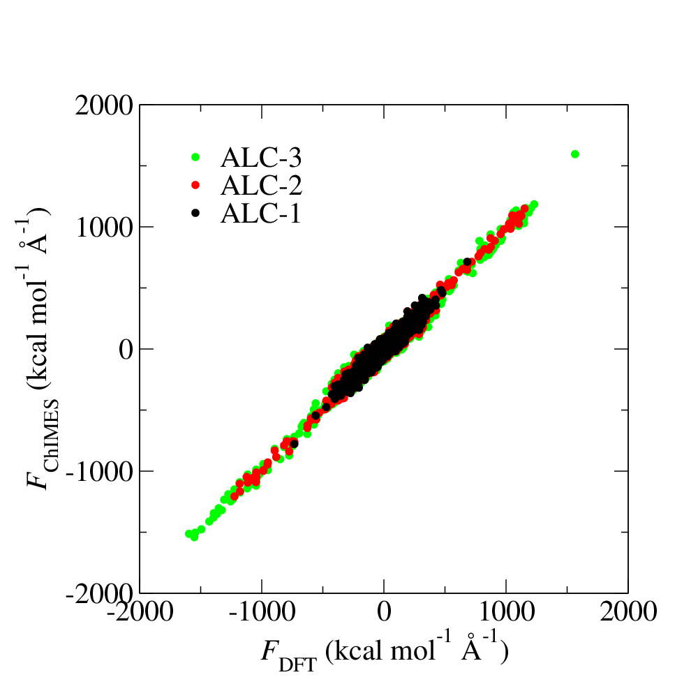
Fig. 2: ALD fitting force pairty plot.

This force parity plot provides DFT-assigned per-atom forces on the x-axis, and corresponding ChIMES predicted forces on the y-axis, in kcal/mol/Angstrom. The ALC-1 data corresponds to data generated by DFT (i.e., the forces contained in liquid_6000K_2.0gcc.xyzf); the ALC-2 data contain everything from ALC-1, as well as forces for the ChIMES-generated configurations selected in step 5 of figure 1, which were assigned DFT forces in step 6 of figure 1. The ALC-3 data is structured similarly.

Next, plot the ALC-{1..3}/CASE-0_INDEP_0/md_statistics.out files. If LAMMPS is used to run molecular dynamics (MD) simulations, plot the etotal values from log.lammps instead. The resulting figure should look like the following:

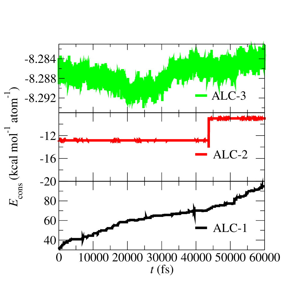
Fig. 3: Conserved quantity for ChIMES molecular dynamics (MD) during ALD iterations.

This figure shows how the conserved quantity varies during ChIMES-MD NVT simulations using the models generated at each ALC. As expected due to the minimal initial training set, dynamics with the ALC-1 model are very unstable (i.e., varying by 55 kcal/mol/atom over 60 ps). Stability is signficantly improved by ALC-2, with the conserved quantity varying by only ~2 kcal/mol/atom. By ALC-3, the model is fully stable, varying by less than .01 kca/mol/atom over the 60 ps trajectory).

---

Additional Examples:

Users can access additional examples in /path/to/ald_driver/examples/.

Example Name	System	Notes
hierarch_fit	carbon/nitrogen	Hierarchical fit for carbon/nitrogen system. See details in this link.
hydrogen	hydrogen	Simple ALD for hydrogen system with 2 cases.
simple_bulk_MFI_cp2k	MFI zeolite	ALD with CP2K with 1 case ran on TACC Stampede3 HPC system.
simple_iter_single_statepoint-cp2k	MFI zeolite	ALD with CP2K with 1 case ran on UM-ARC Greatlakes HPC system.
simple_iter_single_statepoint-MultiNode	MFI zeolite	ALD with CP2K with 3 cases ran on different number nodes for each case.
simple_iter_single_statepoint-lmp-test	molten carbon	ALD with LAMMPS as the MD module and the labeling method with 1 case.
simple_iter_single_statepoint-lmp-test-turbo-test	molten carbon	ALD with LAMMPS for turbo ChIMES fit. Turbo ChIMES functionalities will be included later.

---

In-depth Setup and Options Overview

Setting up Steps 1 & 2

As with a standard ChIMES fit (see e.g, the ChIMES LSQ manual), model generation must begin with selecting an intial training set and specifying fitting hyperparameters. In the ALD, this involves the following files, at a minimum:

<my_fit>/ALL_BASE_FILES/ALC-0_BASEFILES/fm_setup.in
<my_fit>/ALL_BASE_FILES/ALC-0_BASEFILES/traj_list.dat
<my_fit>/ALL_BASE_FILES/ALC-0_BASEFILES/*xyzf
<my_fit>/config.py

The fm_setup.in file is created as usual, except:

• The # TRJFILE # option must be set to MULTI traj_list.dat

• The # SPLITFI # option must be set to false.

See the ChIMES LSQ manual for more information on what these settings control.

Warning

Arbitrary specification of fit hyperparameters (i.e., set in fm_setup.in) will result in inaccurate and/or unstable models. For more information on ChIMES hyperparameters and selection strategies, see:

• The ChIMES LSQ code manual (link)

• R.K. Lindsey, L.E. Fried, N. Goldman, JCTC, 13, 6222 (2017) (link)

• R.K. Lindsey, L.E. Fried, N. Goldman, JCTC 15 436 (2019) (link)

The traj_list.dat file should be structured as usual for ChIMES LSQ, but lines containing the first n-cases entries should have a temperature in Kelvin specified at the very end, where n-cases is the number of statepoints the user would like to simultaneously conduct iterative training to:

3
10 1000K_1.0gcc.xyzf 1000
10 2000K_2.0gcc.xyzf 2000
10 3000K_3.5gcc.xyzf 3000

Note that the above .xyzf files correspond to <my_fit>/ALL_BASE_FILES/ALC-0_BASEFILES/*xyzf.

Finally, options for this first phase of fitting config.py must be specified. A complete set of options and details default values are listed on the ALD Configuration File Options page. Note that for this basic overview we will assume:

• The user is running on a SLURM/SBATCH based HPC system (set by default)

• The HPC system has 36 processors per compute node (set by default)

• We want to generate hydrogen parameters by iteratively fitting at 3 statepoints, simultaneously (indicated by line 6-7).

The example config.py lines necessary for steps 1 & 2 are provided in the code block below. Recalling that ALD functions primarily as a workflow tool, it must be linked with external software. Here, we tell the ALD:

• What element system we are running ALD on (line 7),

• How many statepoints are we fitting to simultaneously (line 8),

• Where the ALD source code is located (line 10),

• Where the ALD will be run (line 11), and

• Where to find our ChIMES_LSQ installation (line 12).

Lines 18-21 tell the ALD where all the files needed to run chimes_lsq are, specifically:

• The ChIMES LSQ input files, fm_setup.in and traj_list.dat (line 18),

• The ChIMES LSQ design matrix generation executable, chimes_lsq (line 19),

• The ChIMES LSQ matrix solution script, chimes_lsq.py (line 20), and

• The ChIMES LSQ parameter file scrubber, post_proc_chimes_lsq.py (line 21).

Finally, lines 25-27 specify how forces, energies, and stresses should be weighted, while lines 29-31 specify how the matrix solution problem should be executed, i.e., using distributed lasso (line 29) with a regularization variable of 1e-8 (line 30), and with a normalized design matrix (line 31). Note that there are many options for these lines, described in detail in the ALD Configuration File Options page.

################################
##### General options
################################

EMAIL_ADD = "<your email>"

ATOM_TYPES     = ["H"]
NO_CASES       = 3

DRIVER_DIR     = "/path/to/al_driver/"
WORKING_DIR    = "/path/to/this/dir/"
CHIMES_SRCDIR  = "/path/to/chimes_lsq/src/"

################################
##### ChIMES LSQ
################################

ALC0_FILES    = WORKING_DIR + "ALL_BASE_FILES/ALC-0_BASEFILES/"
CHIMES_LSQ    = CHIMES_SRCDIR + "../build/chimes_lsq"
CHIMES_SOLVER = CHIMES_SRCDIR + "../build/chimes_lsq.py"
CHIMES_POSTPRC= CHIMES_SRCDIR + "../build/post_proc_chimes_lsq.py"

# Generic weight settings

WEIGHTS_FORCE =   1.0
WEIGHTS_ENER  =   0.1
WEIGHTS_STRES = 100.0

REGRESS_ALG   = "dlasso"
REGRESS_VAR   = "1.0E-8"
REGRESS_NRM   = True

# Job submitting settings (avoid defaults because they will lead to long queue times)

CHIMES_BUILD_NODES = 2
CHIMES_BUILD_QUEUE = "pdebug"
CHIMES_BUILD_TIME  = "01:00:00"

CHIMES_SOLVE_NODES = 2
CHIMES_SOLVE_QUEUE = "pdebug"
CHIMES_SOLVE_TIME  = "01:00:00"

################################
##### Molecular Dynamics
################################

MD_STYLE        = "CHIMES"
CHIMES_MD_MPI   = CHIMES_SRCDIR + "../build/chimes_md"

MOLANAL         = CHIMES_SRCDIR + "../contrib/molanal/src/"
MOLANAL_SPECIES = ["C1"]

################################
##### Single-Point QM
################################

QM_FILES = WORKING_DIR + "ALL_BASE_FILES/QM_BASEFILES"
VASP_QUEUE  = "pdebug"
VASP_EXE = "/path/to/vasp"
VASP_TIME    = "01:00:00"
VASP_NODES   = 2
VASP_PPN     = 36
VASP_MODULES = "mkl intel/18.0.1 impi/2018.0"

---

Setting up Step 3

Step 3 comprises MD simulation with the parameters generated in step 2. Beyond the parameter file, this requires the following at a minimum:

• An initial coordinate file,

• A MD input file specifying the simulation style,

• A MD code executable, and

• Instructions on how to post-process resultant trajectories

Recalling that the current example concerns concurrent iterative fitting for three cases (training state points), this is specified by the following in /path/to/ALL_BASE_FILES/CHIMESMD_BASEFILES/ and config.py, i.e.:

$: ls /path/to//ALL_BASE_FILES/CHIMESMD_BASEFILES/
<my_fit>/ALL_BASE_FILES/CHIMESMD_BASEFILES/case-0.indep-0.input.xyz
<my_fit>/ALL_BASE_FILES/CHIMESMD_BASEFILES/case-0.indep-0.run_md.in
<my_fit>/ALL_BASE_FILES/CHIMESMD_BASEFILES/case-1.indep-0.input.xyz
<my_fit>/ALL_BASE_FILES/CHIMESMD_BASEFILES/case-1.indep-0.run_md.in
<my_fit>/ALL_BASE_FILES/CHIMESMD_BASEFILES/case-2.indep-0.input.xyz
<my_fit>/ALL_BASE_FILES/CHIMESMD_BASEFILES/case-2.indep-0.run_md.in
<my_fit>/ALL_BASE_FILES/CHIMESMD_BASEFILES/bonds.dat

and

################################
##### Molecular Dynamics
################################

MD_STYLE        = "CHIMES"
CHIMES_MD_MPI   = CHIMES_SRCDIR + "chimes_md-mpi"

MOLANAL         = "/path/to/molanlal/folder/"
MOLANAL_SPECIES = ["H1", "H2 1(H-H)", "H3 2(H-H)"]

Each case-*.indep-0.input.xyz is a ChIMES .xyz file containing initial coordinates for the system of interest for the corresponding case, while each case-*.indep-0.run_md.in is the corresponding ChIMES MD input file. Note that case-*.indep-0.run_md.in options # PRMFILE # and # CRDFILE # should be set to WILL_AUTO_UPDATE. For more information on these files, see the (ChIMES LSQ manual). The bonds.dat file will be described below.

In the config.py file snipped above, lines 5 and 6 tell the ALD to use ChIMES MD for MD simulation runs, and provides a path to the MPI-enabled and serial compilations. Lines 9 and 10 provide information on how to post-process the trajectory. Specifically, the ALD will use the a molecular analyzer (“molanal”) to determine speciation for the generated MD trajectories. Once speciation is determined, the ALD will provide a summary of lifetimes and molefractions for species listed in MOLANAL_SPECIES. Note that the species names must match the “Molecule type” fields produced by molanal exactly. These strings are usually determined by running molanal on DFT-MD trajectories, prior to any ALD. Finally, the bonds.dat file specifies bond length and lifetime criteria for molanal. See the molanal readme.txt file for additional information. Be sure to verify specified bonds.dat lifetime criteria are consistent with the timestep and output frequency specified in case-*.indep-0.run_md.in

---

Setting up Step 4

Model validation is purposefully left to the user, as optimal strategies are still an active area of research and are most efficient when application-specific. The user is encouraged to investigate fit performance and physical property recovery on their own.

---

Setting up Step 5

Candidate configuration filtering is conducted in step 5. For basic fitting mode, this simply comprises selecting a subset of configurations generated during the previous MD step for single point evaluation using, e.g., DFT. This is handled entirely automatically by the ALD.

For basic iterative refinement mode, this entails selecting up to 20 evenly spaced configurations from ChIMES-MD simulations at each case, for which all atoms are:

1. Outside the penalty function kick-in region

2. Within the penalty function kick-in region but outside the inner cutoffs

The latter configurations are included to inform the short-ranged region of the interaction potential, which is generally poorly sampled by DFT-MD.

---

Setting up Step 6

Step 6 comprises single point evaluation of configurations selected in step 5 via the user’s requested quantum-based reference method. In this overview, we will assume the user is employing VASP but additional options are described in Options page. To do so, the following must be provided, at a minimum:

<my_fit>/ALL_BASE_FILES/QM_BASEFILES/*.INCAR
<my_fit>/ALL_BASE_FILES/QM_BASEFILES/KPOINTS
<my_fit>/ALL_BASE_FILES/QM_BASEFILES/*.POTCAR

and

################################
##### Single-Point QM
################################

QM_FILES = WORKING_DIR + "ALL_BASE_FILES/QM_BASEFILES"
VASP_EXE = "/path/to/vasp/executable"
VASP_TIME    = "01:00:00"
VASP_NODES   = 2
VASP_PPN     = 36
VASP_MODULES = "mkl intel/18.0.1 impi/2018.0"

There should be one *.INCAR file for each case temperature, i.e. {1000,2000,3000}.INCAR for the present example, with all options set to user desired values for single point evaluation. Note that IALGO = 48 should be used to specifiy the electronic minimization algorithm, and any variable related to restart should be set to the corresponding “new” value. There should also be one .*POTCAR file for each atom type considered, i.e. H.POTCAR for the present example.

Note

Support for additional data labeling schemes (i.e., both quantum- and moleuclar mechanics-based) are incoming.

Tip

The VASP INCAR files provided in ALL_BASE_FILES/QM_BASEFILES for examples using VASP specify either NPAR or NCORE. These values must be consistent with the resources requested in config.py (i.e., VASP_NODES * VASP_PPN). For more details, see the VASP documentation for NPAR and NCORE.

Warning

QM codes can fail to converge in unexpected cases, in manners that are challenging to detect. If you notice your force parity plots indicate generally good model performance but show a few unexpected outliers, verify your QM code is providing the correct answer. This can be done by evaluating the offending configuration with a different code version or a different code altogether.